Heatmap needs "ctc" package from bioconductor, to install "ctc" package:

>source("http://bioconductor.org/biocLite.R")
>biocLite("ctc")

heatmap(...) function can draw a heatmap, it's usage is:

heatmap(x, Rowv=NULL, Colv=if(symm)"Rowv" else NULL,
distfun = dist, hclustfun = hclust,
reorderfun = function(d,w) reorder(d,w),
add.expr, symm = FALSE, revC = identical(Colv, "Rowv"),
scale=c("row", "column", "none"), na.rm = TRUE,
margins = c(5, 5), ColSideColors, RowSideColors,
cexRow = 0.2 + 1/log10(nr), cexCol = 0.2 + 1/log10(nc),
labRow = NULL, labCol = NULL, main = NULL,
xlab = NULL, ylab = NULL,
keep.dendro = FALSE, verbose = getOption("verbose"), ...)

x: Numeric matrix
Rowv: Row dendrogram
Colv: Column dendrogram
...

Let's first have a look of our data file named heatmap.csv:

elements S1 S2 S3 S4 S5 S6 S7 S8
R1 -0.0027 0.1057 0.1976 0.0209 0 0.0089 0.0082 0.0209
R2 0 -0.1204 0.2627 0 0 0.283 0.2076 -0.0158
R3 0 -0.1204 0.2627 0 0 0.283 0.2076 -0.0158
R4 0.0142 0 -0.454 0.0101 -0.0213 -0.0084 -0.0121 0.0083
R5 0 0 -0.2334 0.007 0.4151 0 0.0987 0.021
R6 0.0381 0.0644 0.2302 0 0 -0.0476 0.2432 -0.0069
R7 0.0381 0.0644 0.2302 0 0 -0.0476 0.2432 -0.0069
R8 0.0381 0.0644 0.2302 0 0 -0.0476 0.2432 -0.0069
R9 0.0891 -0.1022 -0.4466 -0.4877 -0.0175 -0.0523 -0.4792 -0.0547
R10 0.0046 -0.1539 -0.4645 0 -0.0282 0 -0.0217 0.017
R11 0.0706 0.028 0.3626 0 0.0196 -0.0094 0.3086 0
R12 0.0311 0.0759 0.2119 0 -0.0022 0 0 0.0117
R13 0.0013 0.0702 -0.3176 0.0152 0.0095 -0.0224 0.2069 0.005
R14 0.0491 0.0525 -0.4329 0.0237 -0.0038 -0.0224 0.2065 0.005
R15 0.0256 0.0579 0.1846 0.0024 0.0029 -0.0165 0.4781 -0.0123
R16 -0.0061 -0.1554 -0.0635 0.0121 -0.0282 0 -0.016 0.017
R17 -0.0061 -0.1554 -0.0635 0.0121 -0.0282 0 -0.016 0.017

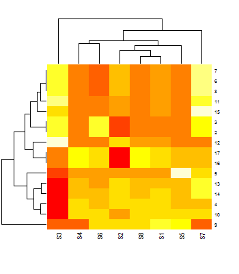
Let's draw a simple heatmap:

>x <- read.csv("heatmap.csv", header=T, dec=".",sep=",")
>imageVals <- as.matrix(cn[2:nrow(x),2:ncol(x)]);
>heatmap(imageVals)

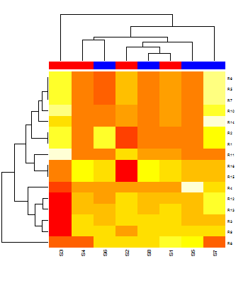
For further improvement, we's like to replace the rownames at the right side with names in the first column of the file. Suppose S1-S4 come from location A, and s5-S8 come from location B, we will marked it as red and blue color as a bar under the top dendrogram.

>rowNames = x[,1];
>samplecolors <- c("red","red","red","red","blue","blue","blue","blue");
>heatmap(imageVals,labRow=rowNames,ColSideColors=as.vector(samplecolors))